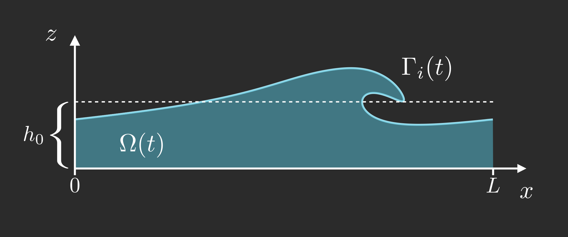
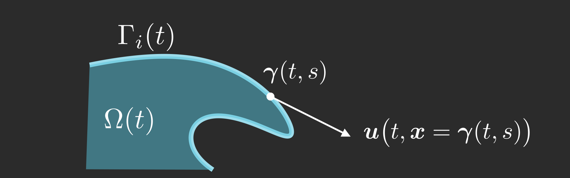
Definition
The free surface \( \boldsymbol{\gamma} \) is said to have broken at time \(t \geq 0\) if \( \partial_s\gamma_x(t,\cdot) = \partial_s X_t \) fails to be invertible at some point.
Superharmonic Instability
Longuet-Higgins (1978)
Longuet-Higgins & Cokelet (1978)
⤷ using the numerical method of Longuet-Higgins & Cokelet (1976)
Later confirmed and extended by:
Tanaka (1983, 1985)
Tanaka, Dold, Lewy & Peregrine (1987)
Effects of viscosity and surface tension:
Mansar, Turner, Bridges & Dias (2025)
The geometric viewpoint
- To compute the shape of the wave
- Explicit interface representation
- Lagrangian advection
- Fails as the splash singularity occurs
The phenomenological viewpoint
- To compute the energy dissipation
- Implicit interface representation
- Eulerian advection
- Mostly two-fluids studies
Analtical result: Masmoudi & Rousset (2017) Uniform Regularity and Vanishing Viscosity Limit for the Free Surface Navier–Stokes Equations
On the vanishing viscosity limit up to the splash
\[\mathrm{Re} \to +\infty \]
- A numerical method for the free-surface Navier-Stokes equations
- Finite Element method
- Arbitrary Lagrangian-Eulerian advection
- Boundary layers in Water Waves
- The free-surface boundary layer
- Vorticity separation from the bed
Euler (+ irrotationality)
-
Mapping to the unit circle in \(\mathbb{C}\):
⤷Longuet-Higgins & Cokelet (1976) -
The vortex and dipole methods:
⤷Baker, Meiron & Orszag (1982)
⤷Baker & Xie (2011)
⤷Dormy & Lacave (2024) -
Boundary Element Methods (BEM) in 3D:
⤷Grilli, Guyenne & Dias (2001)
Navier-Stokes
-
Two-dimensional studies:
⤷Chen, Kharif, Zaleski & Li (1999)
⤷Deike, Popinet & Melville (2015) -
Three-dimensional studies:
⤷Lubin & Glockner (2015)
⤷Deike, Melville & Popinet (2016)
⤷Mostert, Popinet & Deike (2022) ⤷Scapin et al. (2025)
Non-dimensional quantities: \[ \begin{align} \boldsymbol{x} & \to h_0 \boldsymbol{x} \\ \boldsymbol{u} & \to \sqrt{gh_0} \boldsymbol{u} \\ p & \to \rho g h_0 p \\ \end{align} \] yielding the following Reynolds number, \[ \mathrm{Re} = \frac{h_0 \sqrt{gh_0}}{\nu} \]
Incompressible, non-dimensional Navier-Stokes equations in \(\Omega(t)\) \[ \begin{align} \partial_t \boldsymbol{u} + \boldsymbol{u} \cdot \boldsymbol{\nabla} \boldsymbol{u} &= - \boldsymbol{\nabla}p + \frac{1}{\mathrm{Re}}\, \Delta \boldsymbol{u} + \boldsymbol{g} \\ \boldsymbol{\nabla} \cdot \boldsymbol{u} &= 0 \end{align} \]
Stress-free boundary condition on the free surface \[ \begin{align} p \hat{\boldsymbol{n}} - \frac{1}{\mathrm{Re}} \, \Big[ \boldsymbol{\nabla} \boldsymbol{u} + \big(\boldsymbol{\nabla}\boldsymbol{u}\big)^{\top} \Big] \, \hat{\boldsymbol{n}} &= 0 && \text{on } \Gamma_i(t) \end{align} \] Navier boundary condition on the bottom topography \(\Gamma_b = \{z = 0\}\) \[ \begin{align} \hat{\boldsymbol{\tau}}\,\Big[\boldsymbol{\nabla} \boldsymbol{u} + \big(\boldsymbol{\nabla}\boldsymbol{u}\big)^{\top}\Big] \, \hat{\boldsymbol{n}} &= 0 & u_z &= 0 \end{align} \]
We use the first order (in \(a\)) solution (i.e. a linear wave) of amplitude \(a = 0.5\), \[ \boldsymbol{\gamma}(t=0,s) = \begin{bmatrix} s \\ h_0 + a \cos(kx) \end{bmatrix}\qquad\text{and}\qquad \boldsymbol{u}_0(x,z) = \frac{a\omega}{\sinh(kh_0)} \begin{bmatrix} \cosh(k\style{color: #42affa;}{h_0}) \cos(kx) \\ \sinh(k\style{color: #42affa;}{h_0}) \sin(kx) \end{bmatrix} \] Then we solve numerically the following elliptic problem,
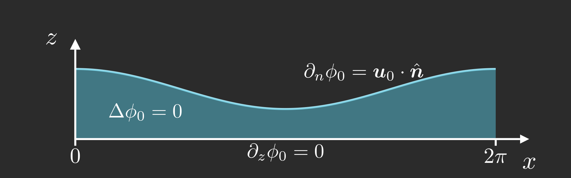
At last, the initial velocity is computed as \( \boldsymbol{u}(t = 0) = \boldsymbol{\nabla} \phi_0 \)
We represent the free surface as a parametrised curve \( \boldsymbol{\gamma}(t,s) \) whose points are advected in a Lagrangian manner, \[ \partial_t \boldsymbol{\gamma}(t,s) = \boldsymbol{u}\big( t, \boldsymbol{x} = \boldsymbol{\gamma}(t,s) \big) \]
We use the FreeFEM library Hecht (2012) to
- generate and handle the mesh
- build and handle the matrices
- use the PETSc methods easily
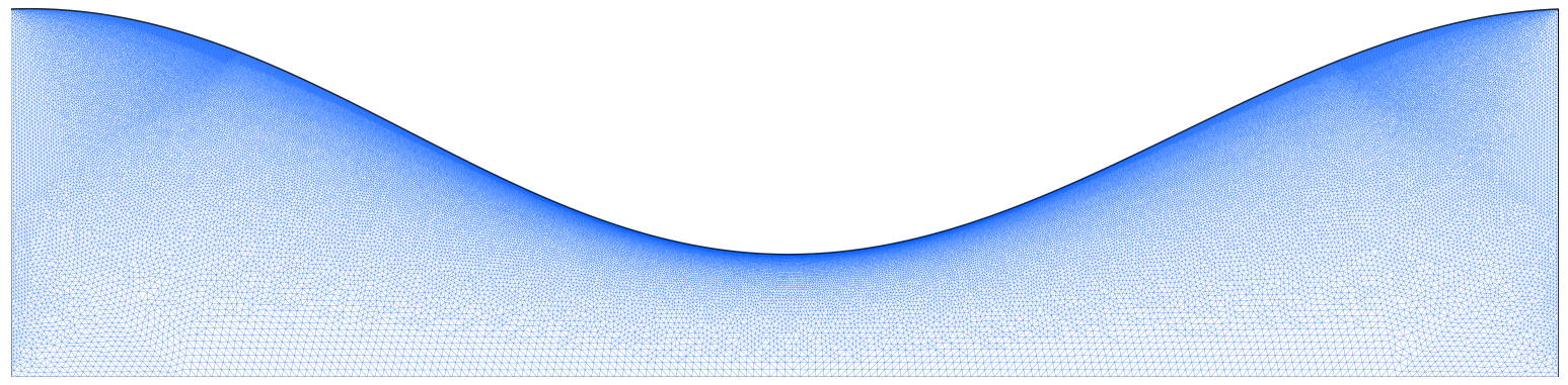
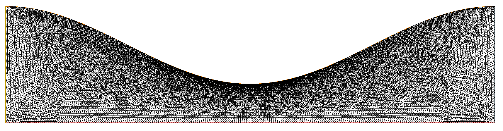
Figure - The mesh generated from the initial free surface (\(\approx 200\,000\) triangles).
We define the function space used for the velocity \[ \mathbf{H}^1_{\Gamma_b} = \Big\{ \boldsymbol{v} \in H^1\big( \Omega(t) ; \mathbb{R}^2 \big) \text{ s.t. } \boldsymbol{v} \cdot \hat{\boldsymbol{n}} = 0 \text{ on } \Gamma_b \Big\} \] Note that the incompressibility is not assumed in the function space.
Find \( (\boldsymbol{u}, p) \) such that, \[ \int_{\Omega(t)} \boldsymbol{v} \cdot \partial_t \boldsymbol{u} + \boldsymbol{v} \cdot \big( \boldsymbol{u} \cdot \boldsymbol{\nabla} \boldsymbol{u} \big) + \frac{2}{\mathrm{Re}}\, \mathsf{S}(\boldsymbol{v}):\mathsf{S}(\boldsymbol{u}) - p \boldsymbol{\nabla}\cdot\boldsymbol{v} + q \boldsymbol{\nabla}\cdot\boldsymbol{u} - \boldsymbol{v} \cdot \boldsymbol{g} = 0 \] for all \( (\boldsymbol{v}, q) \) and at all time \(t\in(0,T)\).
We define the function space used for the velocity \[ \mathbf{H}^1_{\Gamma_b} = \Big\{ \boldsymbol{v} \in H^1\big( \Omega(t) ; \mathbb{R}^2 \big) \text{ s.t. } \boldsymbol{v} \cdot \hat{\boldsymbol{n}} = 0 \text{ on } \Gamma_b \Big\} \] Note that the incompressibility is not assumed in the function space.
Find \( (\boldsymbol{u}, p) \) such that, \[ \int_{\Omega(t)} \boldsymbol{v} \cdot \partial_t \boldsymbol{u} + \boldsymbol{v} \cdot \big( \boldsymbol{u} \cdot \boldsymbol{\nabla} \boldsymbol{u} \big) + \frac{2}{\mathrm{Re}}\, \mathsf{S}(\boldsymbol{v}):\mathsf{S}(\boldsymbol{u}) - p \boldsymbol{\nabla}\cdot\boldsymbol{v} + q \boldsymbol{\nabla}\cdot\boldsymbol{u} - \boldsymbol{v} \cdot \boldsymbol{g} = \frac{1}{\mathrm{Bo}} \int_{\Gamma_i(t)} \kappa \boldsymbol{v} \cdot \hat{\boldsymbol{n}} \] for all \( (\boldsymbol{v}, q) \) and at all time \(t\in(0,T)\).
The Arbitrary Lagrangian-Eulerian Method (ALE)
In our case, we compute the mesh's velocity by numerically solving the following elliptic problem at each time step, \[ \left\{ \begin{array}{rcll} \Delta \boldsymbol{w} &=& 0 & \text{in the domain } \Omega(t) \\ \boldsymbol{w} &=& \boldsymbol{u} & \text{on the free surface } \Gamma_i(t) \\ \boldsymbol{w} &=& 0 & \text{on the bottom } \Gamma_b \\ \end{array} \right. \]
We use a backward Euler (implicit) scheme for all terms but the non-linearity, \[ \frac{\boldsymbol{u}^{n+1} - \boldsymbol{u}^{n}}{\delta t} + (\boldsymbol{u}^{n} - \boldsymbol{w}^{n}) \cdot \boldsymbol{\nabla} \boldsymbol{u}^{n+1} = - \boldsymbol{\nabla} p^{n+1} + \frac{1}{\mathrm{Re}}\, \Delta \boldsymbol{u}^{n+1} - \hat{\boldsymbol{z}} \] \[ \boldsymbol{\nabla} \cdot \boldsymbol{u}^{n+1} = 0 \]
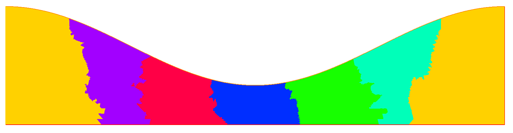
Figure - Sample domain decomposition with 6 MPI processes.
Figures - Sample domain decomposition with 6 MPI processes.
On the vanishing viscosity limit up to the splash
\[\mathrm{Re} \to +\infty \]
- A numerical method for the free-surface Navier-Stokes equations
- Finite Element method
- Arbitrary Lagrangian-Eulerian advection
- Boundary layers in Water Waves
- The free-surface boundary layer
- Vorticity separation from the bed
Animated Figure (from R. & Dormy (2024)) - Interface evolution for a Reynolds number \(\mathrm{Re} = 10^6\)
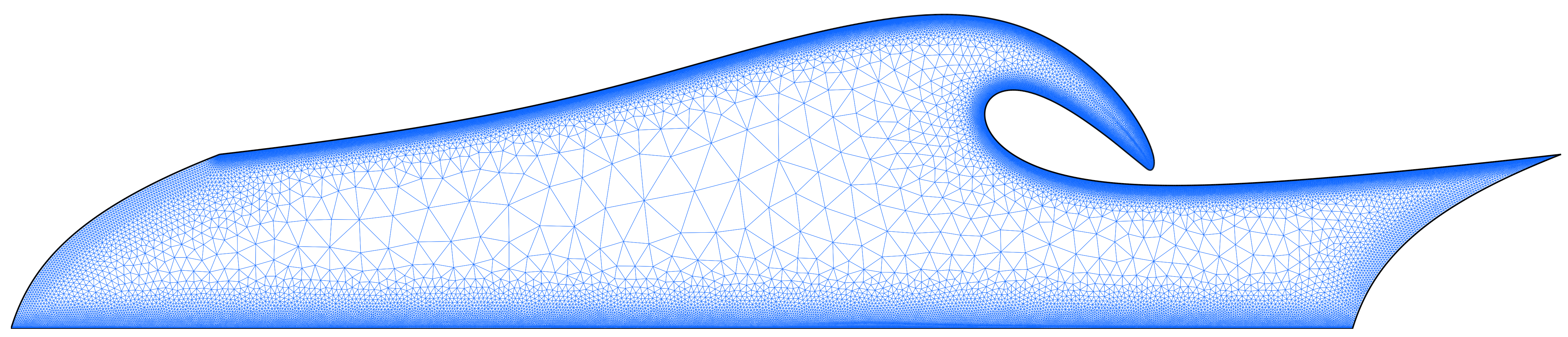
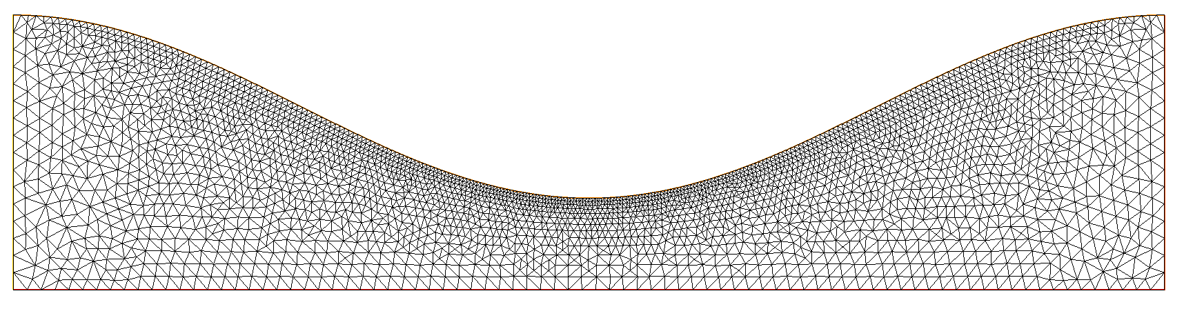
Figure - The mesh close to the end of the simulation shown before.
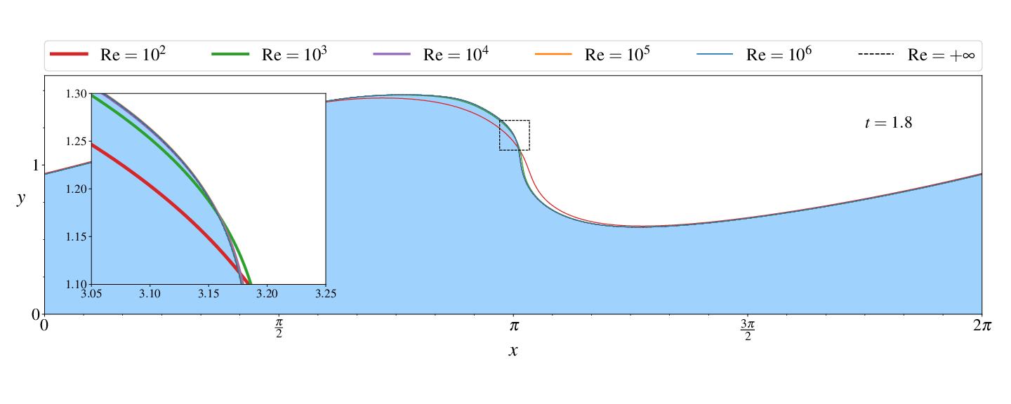
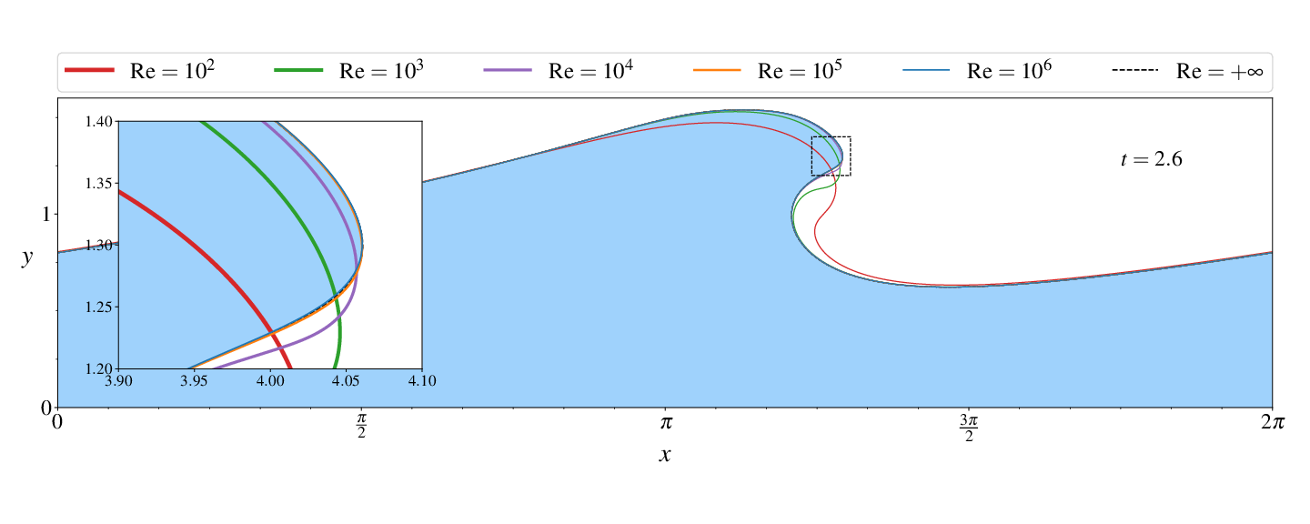
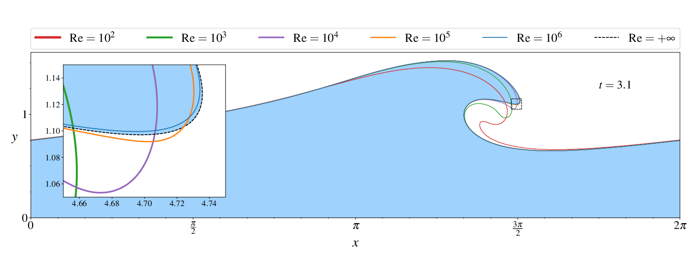
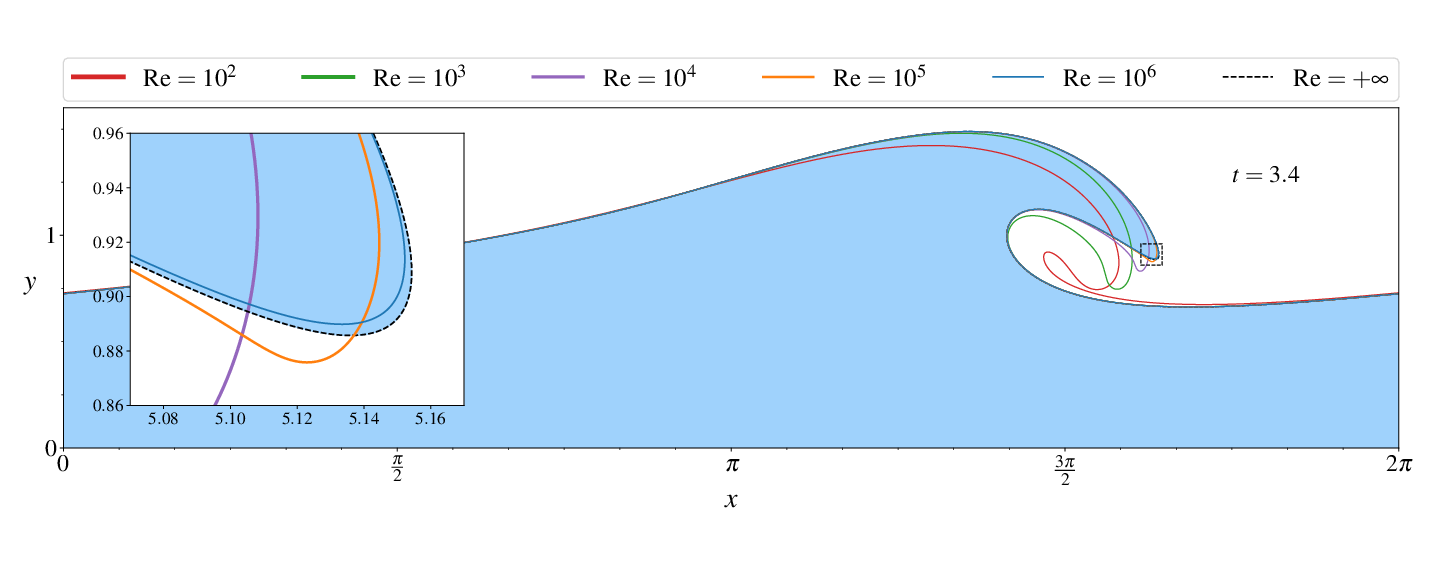
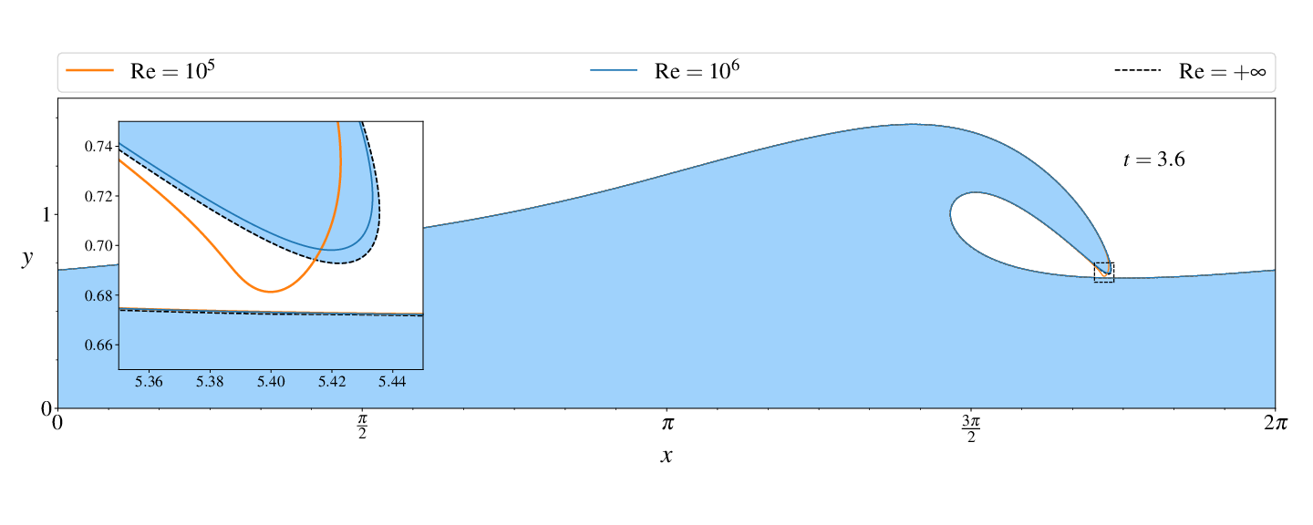
Figures (from R. & Dormy (2024)) - Convergence to the inviscid solution (computed using the numerical method of Dormy & Lacave (2024) )
A local equation for the kinetic energy can be obtained directly from the Navier-Stokes system, \[ \frac{\mathrm{D}}{\mathrm{D}t} \left( \frac{\boldsymbol{u}^2}{2} \right) = \boldsymbol{u} \cdot \boldsymbol{g} - \boldsymbol{u}\cdot \boldsymbol{\nabla} p \style{color: #42affa;}{\ - \frac{1}{\mathrm{Re}}\, \Big[ \boldsymbol{\nabla}\cdot \big( \boldsymbol{u}^{\perp} \omega \big) + \omega^2 \Big]} \] with \( \boldsymbol{u}^{\perp} = [-u_y, u_x] \). The dissipation arises in the support of the vorticity \(\omega\).
Generation of vorticity can be understood in light of the stress-free boundary condition, \[ \begin{align} p \hat{\boldsymbol{n}} - \frac{1}{\mathrm{Re}} \, \Big[ \boldsymbol{\nabla} \boldsymbol{u} + \big(\boldsymbol{\nabla}\boldsymbol{u}\big)^{\top} \Big]\, \hat{\boldsymbol{n}} = 0 \qquad & \Longrightarrow \qquad \hat{\boldsymbol{\tau}} \, \Big[ \boldsymbol{\nabla} \boldsymbol{u} + \big(\boldsymbol{\nabla}\boldsymbol{u}\big)^{\top} \Big]\, \hat{\boldsymbol{n}} = 0 \\ & \Longrightarrow \qquad \omega = 2 \kappa \big( \boldsymbol{u} \cdot \hat{\boldsymbol{\tau}} \big) - 2 \partial_s \big( \boldsymbol{u} \cdot \hat{\boldsymbol{n}} \big) \end{align} \]
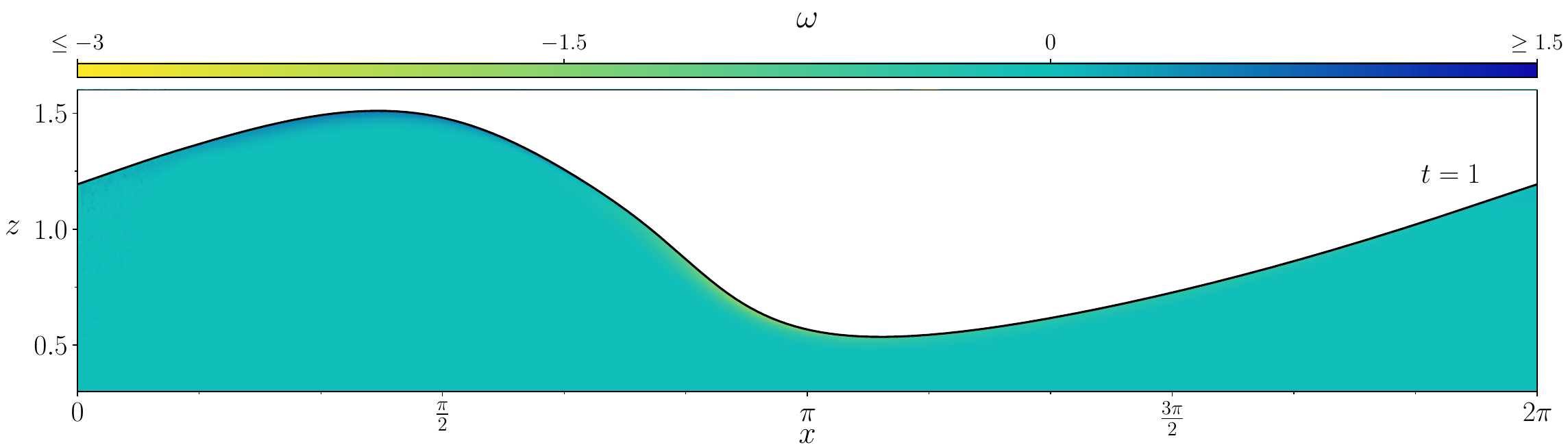
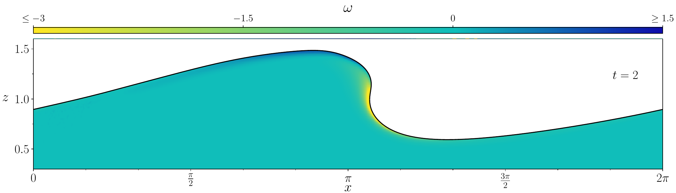
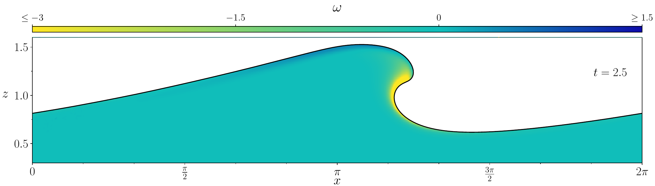
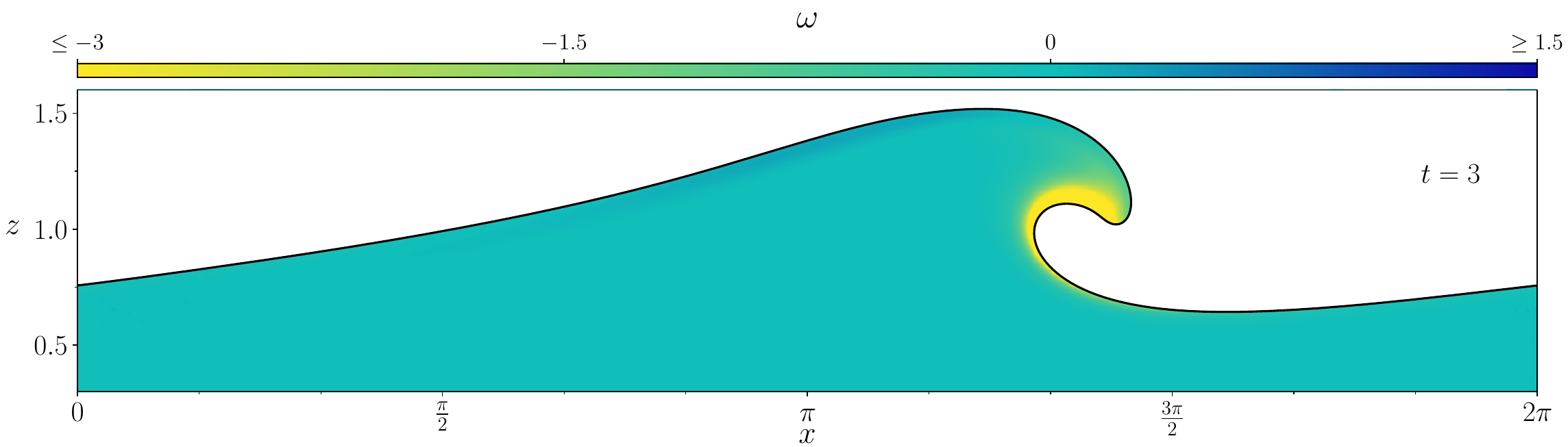
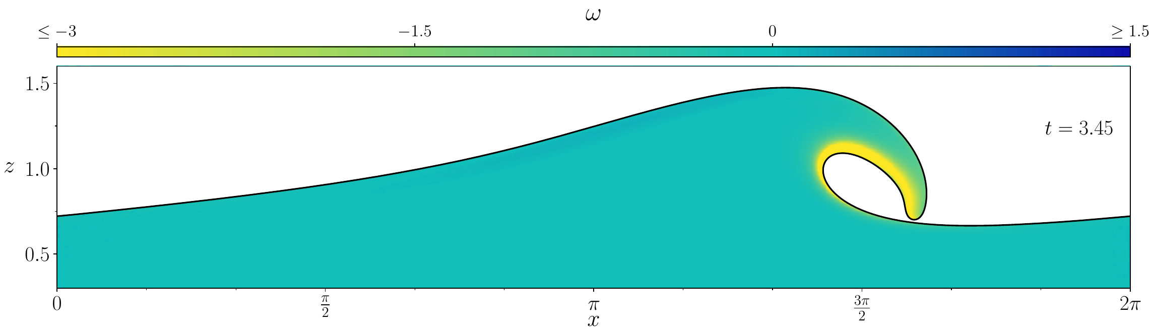
Figures (from R. & Dormy (2024)) - The vorticity generated during the \(\mathrm{Re} = 10^3\) simulation.
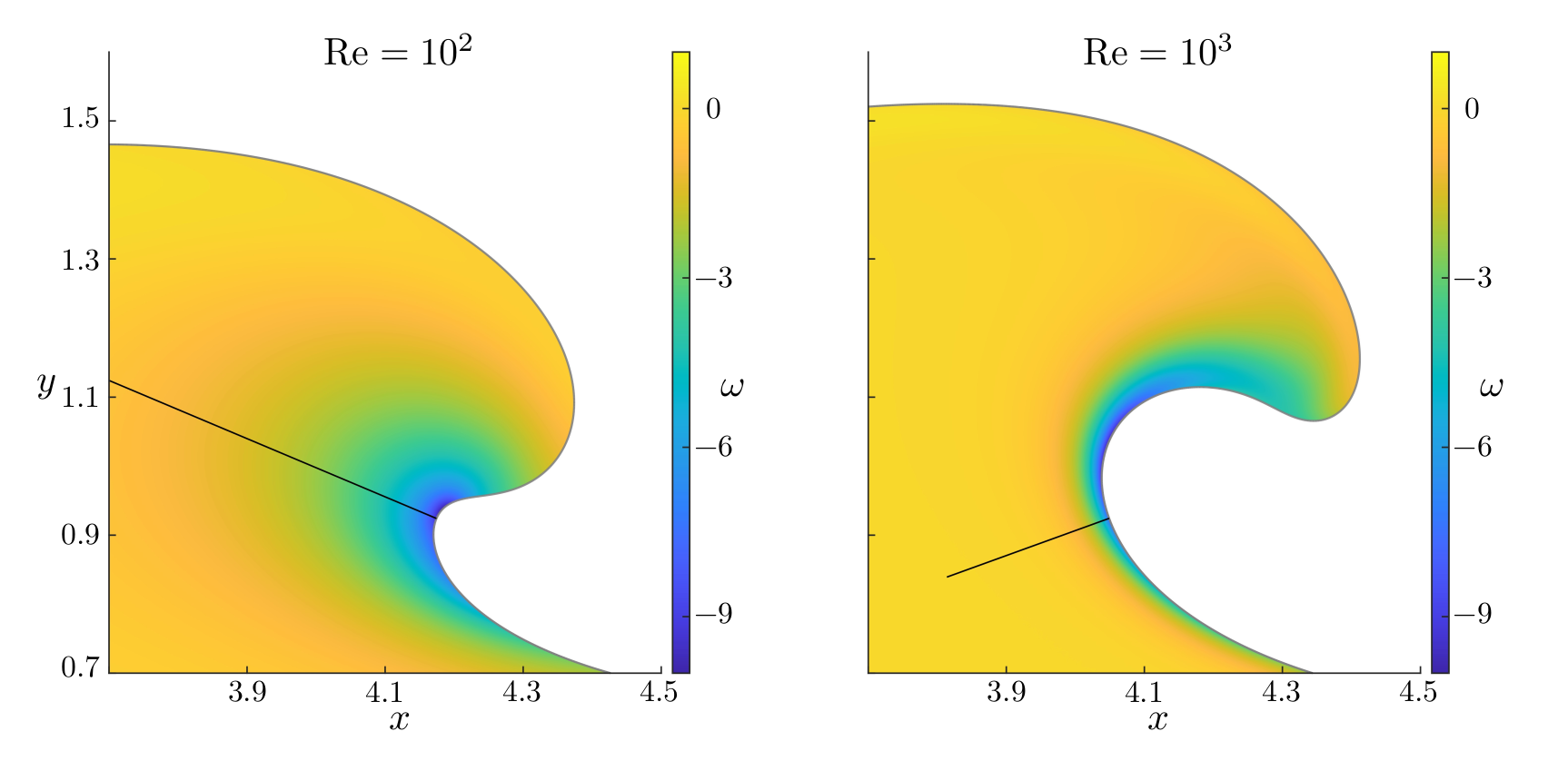
Figures (from R. & Dormy (2024)) - Close-up on the Boundary Layer at time \(t = 2.9\)
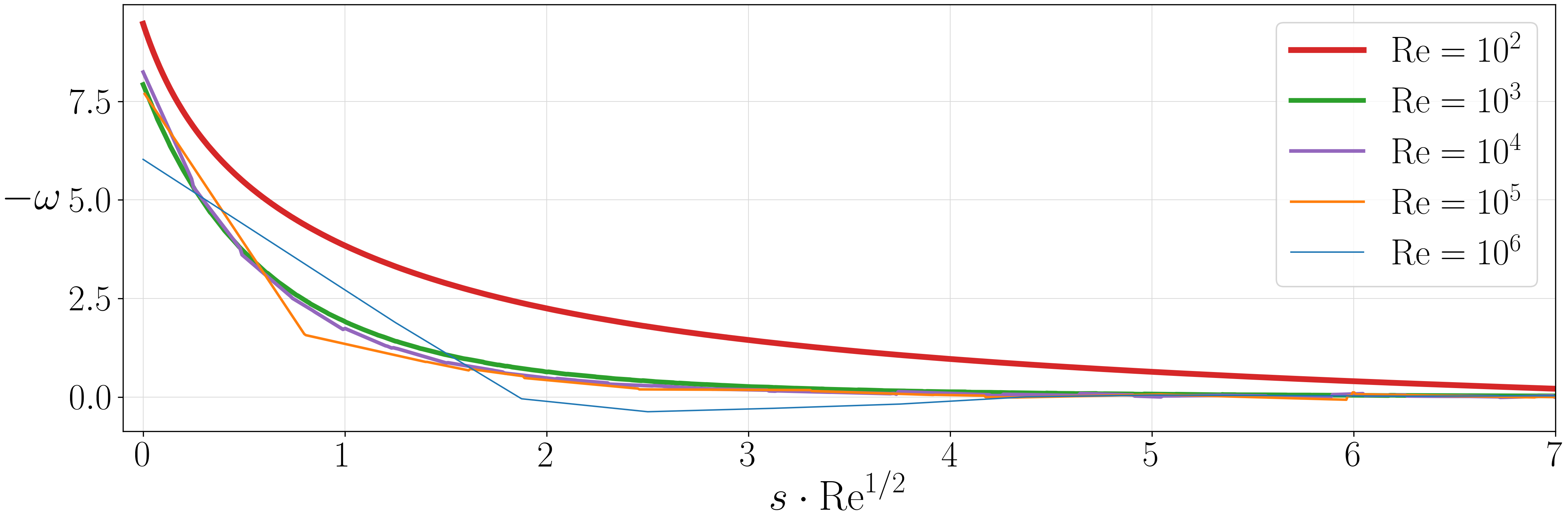
Figure (from R. & Dormy (2024)) - Corresponding vorticity cross section.
Stress-free boundary condition on the free surface \[ \begin{align} p \hat{\boldsymbol{n}} - \frac{1}{\mathrm{Re}} \, \Big[ \boldsymbol{\nabla} \boldsymbol{u} + \big(\boldsymbol{\nabla}\boldsymbol{u}\big)^{\top} \Big] \, \hat{\boldsymbol{n}} &= 0 && \text{on } \Gamma_i(t) \end{align} \] Navier/free-slip No-slip/Dirichlet boundary condition on the bottom topography \(\Gamma_b\), \[ \boldsymbol{u} = 0\qquad\text{on } \Gamma_b \]
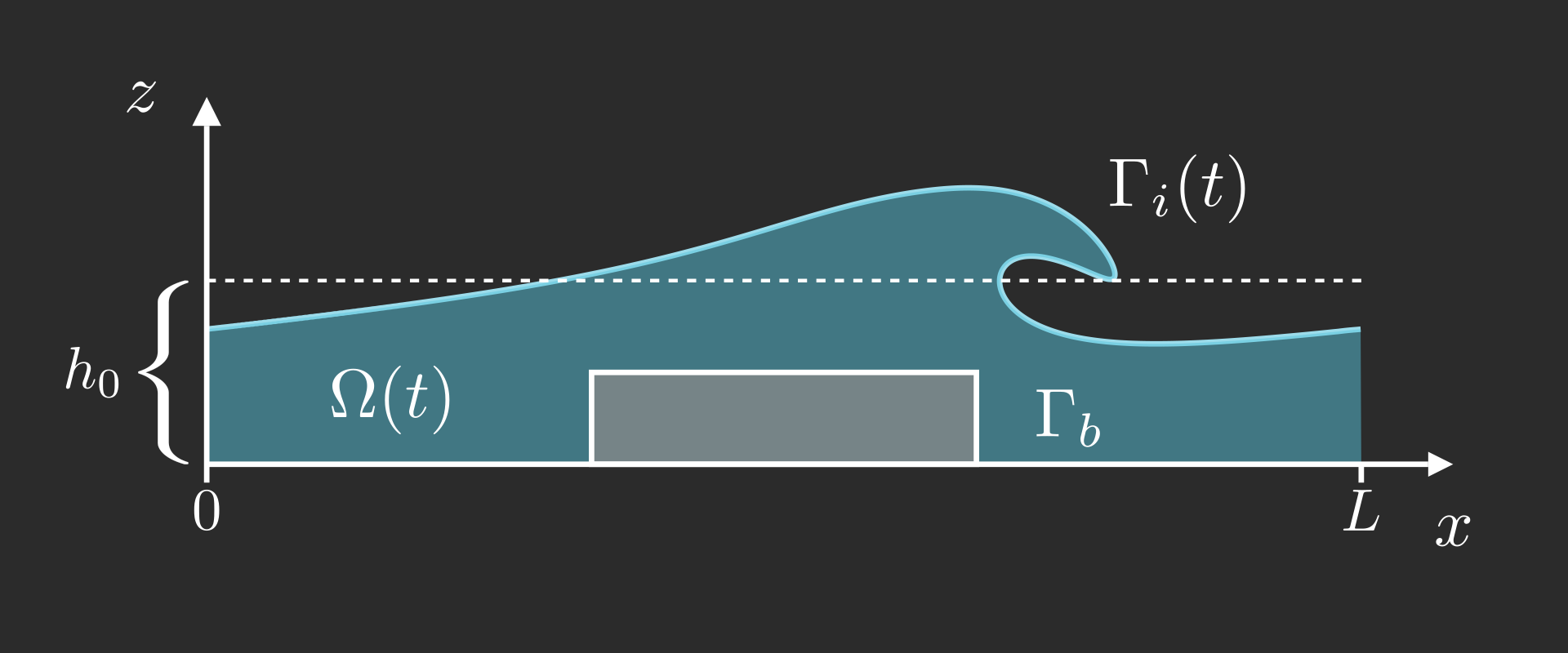
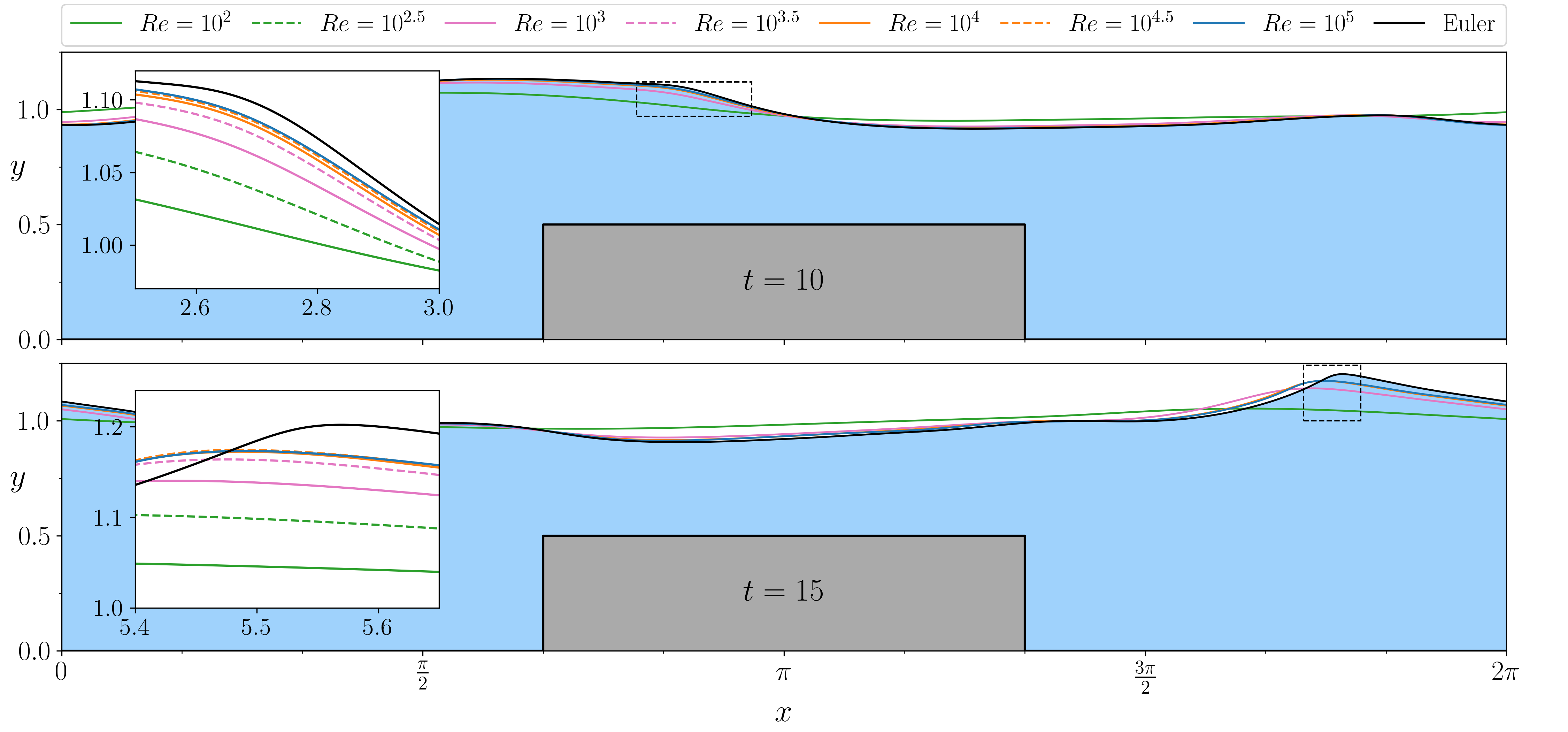
Figure (from R. & Dormy (2026)) - Free surfaces for different values of Reynolds' number \(\mathrm{Re}\). The "Euler" result has been computed using the numerical method of Dormy & Lacave (2024).
Animated Figure (from R. & Dormy (2026)) - Vorticity evolution for a Reynolds number \(\mathrm{Re} = 10^5\).
Phenomenon already observed by Lin & Huang (2010)
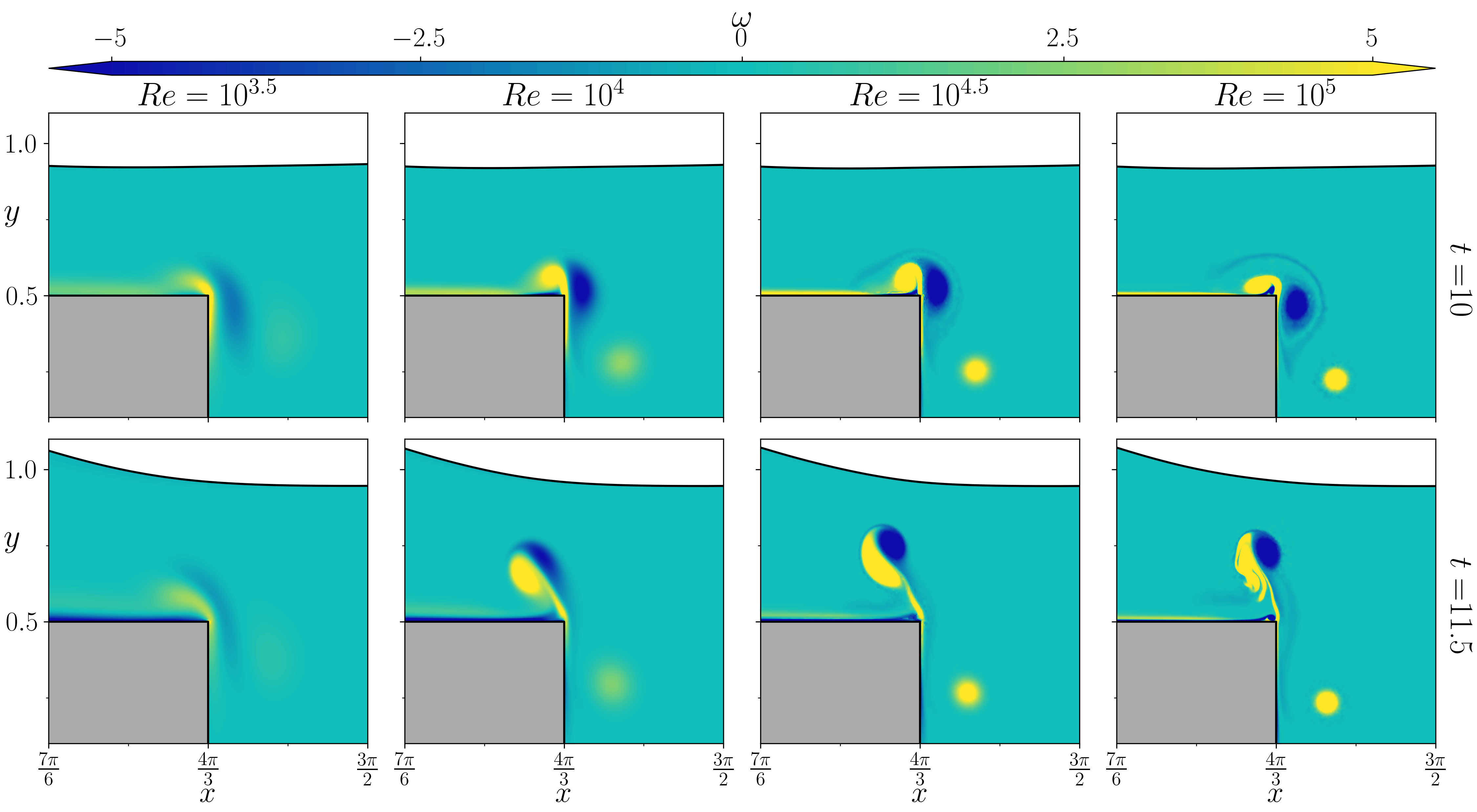
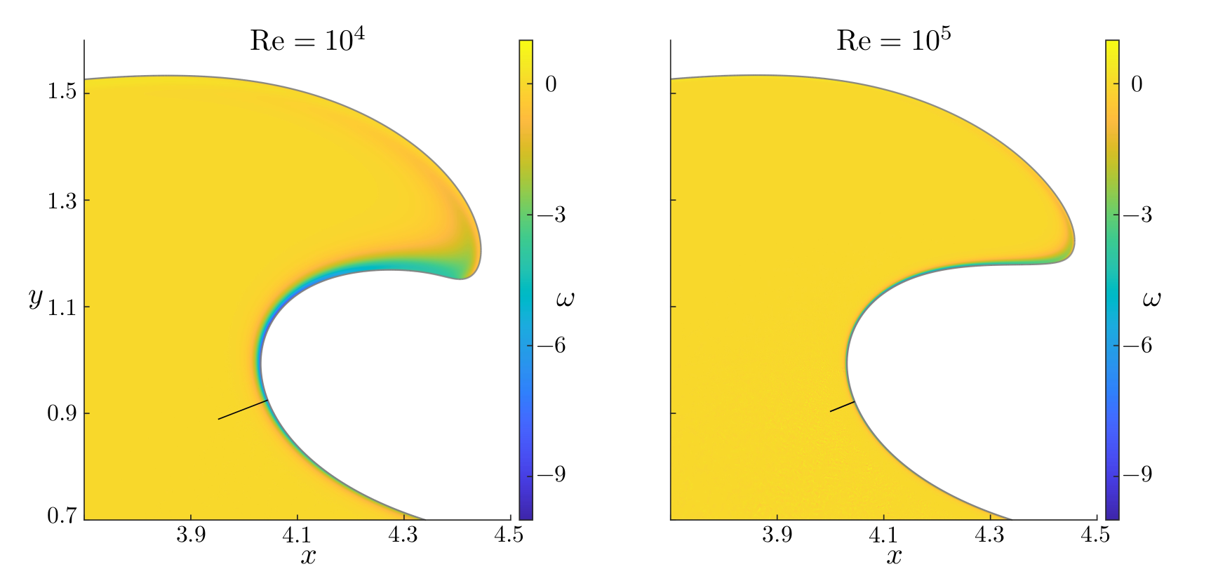
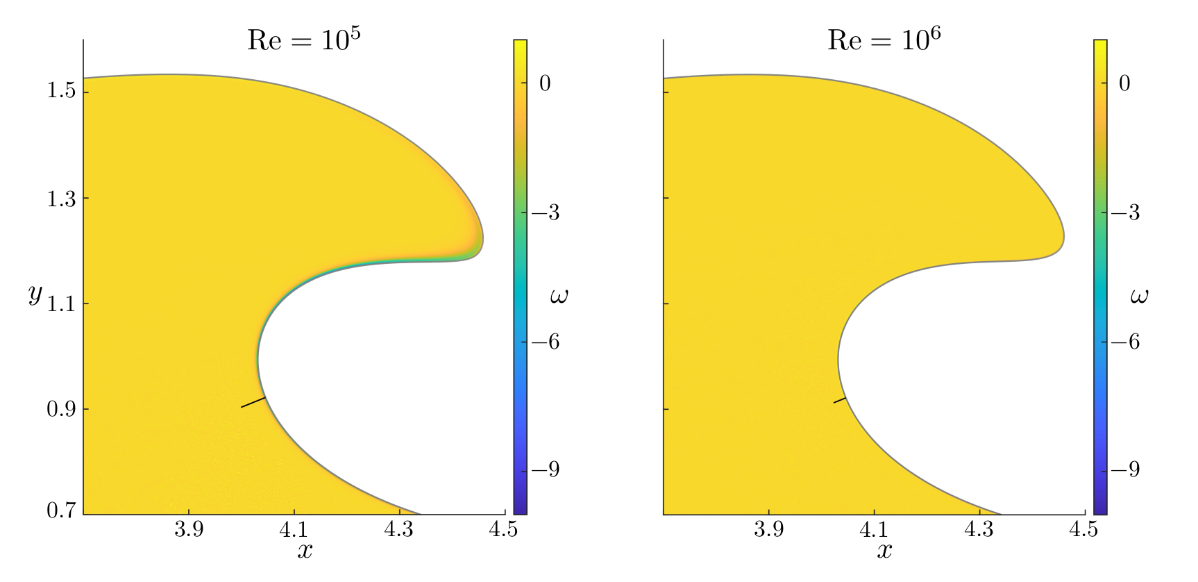
Figures (from R. & Dormy (2026)) - The vorticity at fixed times \(t = 10\) and \(t = 11.5\) for \(\mathrm{Re} = 10^{3.5}\), \(10^4\), \(10^{4.5}\) and \(10^5\).
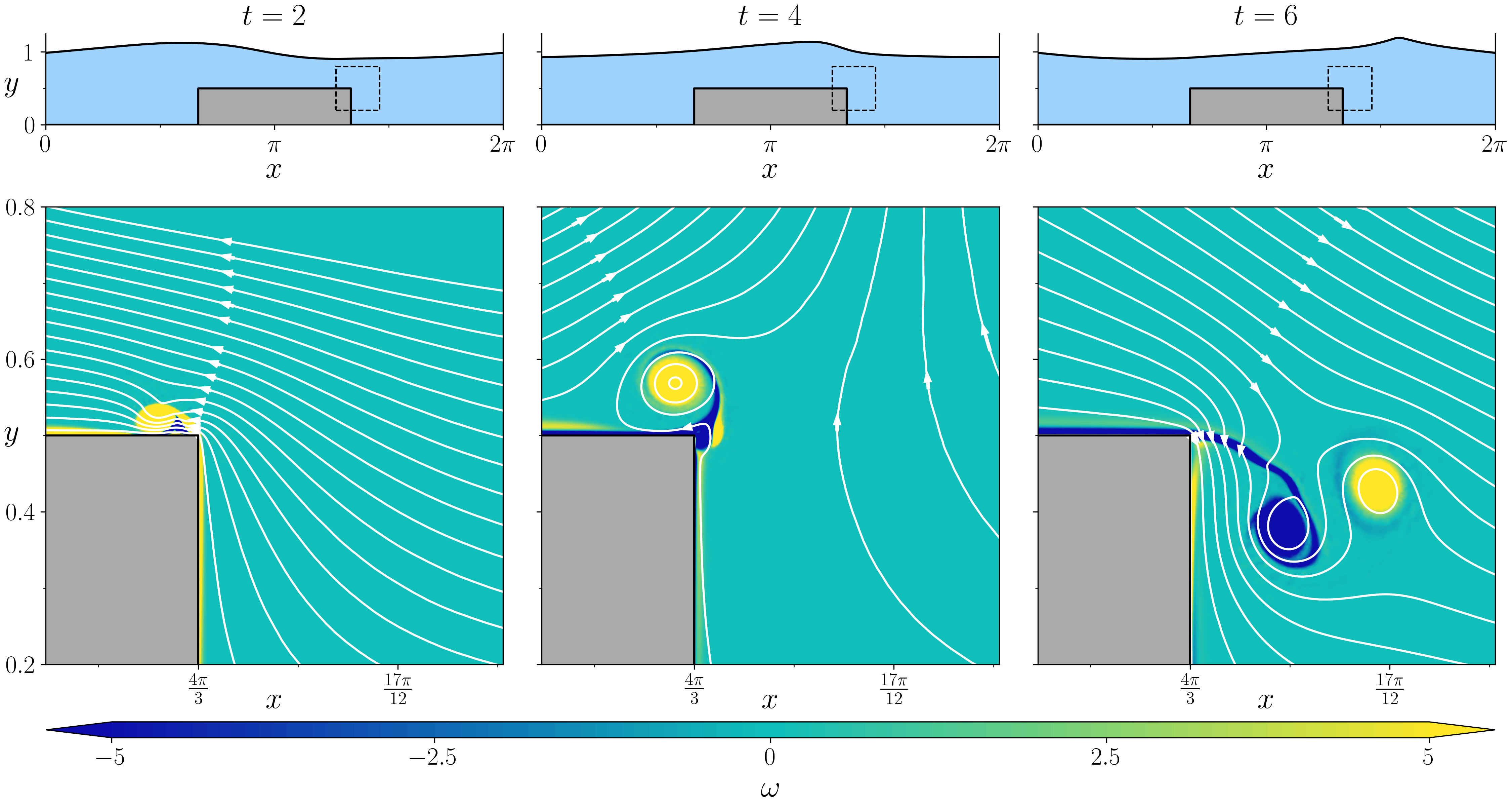
Figure (from R. & Dormy (2026)) - Streamlines at \(\mathrm{Re} = 10^5\).
Animated Figure (from R. & Dormy (2026)) - Vorticity evolution at \(\mathrm{Re} = 10^5\).
Animated Figure (from R. & Dormy (2026)) - Vorticity evolution at \(\mathrm{Re} = 10^5\).
Animated Figure (from R. & Dormy (2026)) - Vorticity evolution at \(\mathrm{Re} = 10^5\).
Animated Figure (from R. & Dormy (2026)) - Vorticity evolution at \(\mathrm{Re} = 10^5\).
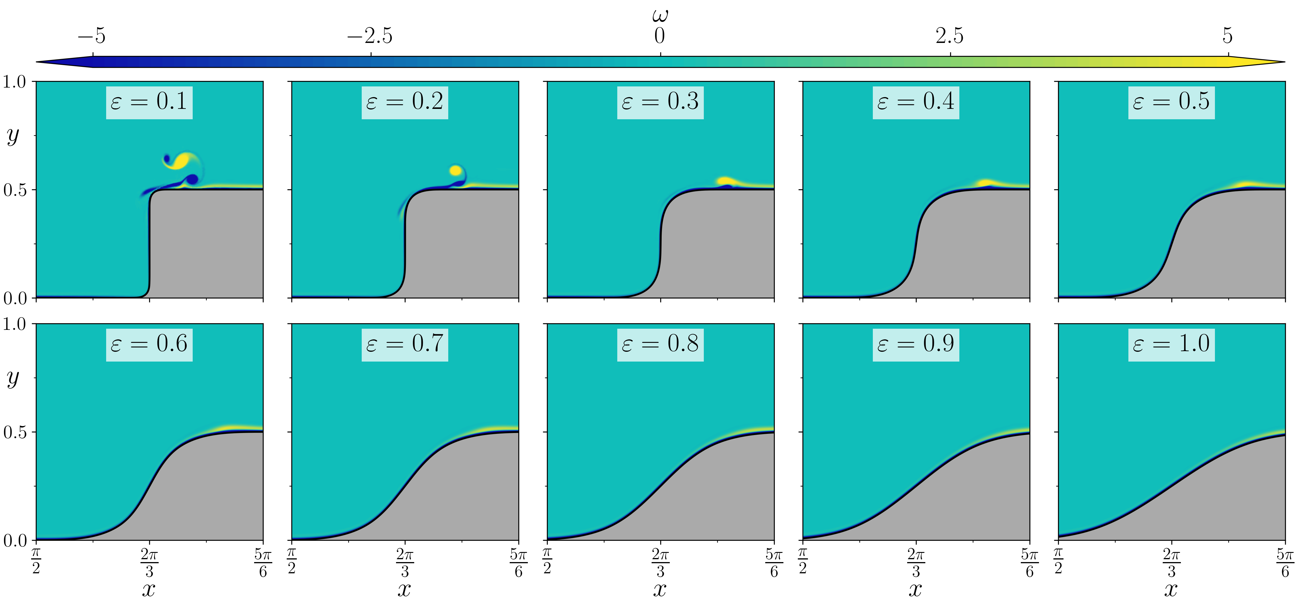
Figure (from R. & Dormy (2026)) - Vorticity at fixed time \(t = 10\) with different curvature radii \(\varepsilon\).
- Mathematical justification of the ALE method
- 3D Navier-Stokes code
- 3D Euler code (Boundary Elements)
Animated Figure - 3D Interface evolution at a Reynolds number \(\mathrm{Re} = 10^4\).
Thank you for your attention!
Slides created using reveal.js
Drawings & animations created using Manim Community
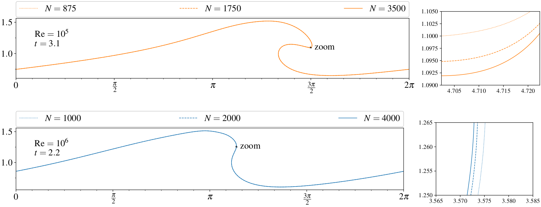
Figure - Numerical convergence